Vertica K-Means 聚类算法实战

原文：K-Means Clustering Using Vertica's In-Built Machine Learning Functions 数据集：Iris（150 条记录，4 个数值特征，3 个品种） 说明：中文注释 + 完整实验过程 + 全部 SQL 原文

概述

K-means 是最流行的聚类算法之一。它将数据分为 K 个组（簇），使得组内样本相似度高、组间差异大。属于无监督学习，即算法仅根据数据特征自行寻找分组，无需标签。

典型应用：电商用户浏览/购买行为分群，用于推荐系统。

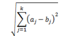
欧几里德距离

K-means 基于欧几里德距离（Euclidean distance）衡量样本间相似度，这是最常用的统计距离度量之一。在二维空间中即为两点间的直线距离：

算法步骤

1. 随机将数据点分配到 K 个簇，初始化 K 个簇质心（centroid）
2. 对每个观测值，计算其到每个簇质心的欧几里德距离，将其归入最近的簇
3. 重新计算新簇的质心（即簇内各点均值）
4. 重复步骤 2 和 3，直到质心不再变化

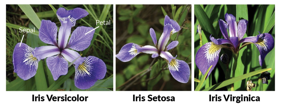
数据集：Iris（鸢尾花）

Iris 数据集包含 150 条记录、4 个数值特征（花萼长度/宽度、花瓣长度/宽度）、3 个品种标签（Setosa、Versicolor、Virginica）。其中 Setosa 与其他两个品种线性可分，而 Versicolor 和 Virginica 之间不完全线性可分。

数据加载

mldb=> CREATE TABLE iris_train (
    id int, Sepal_Length float, Sepal_Width float,
    Petal_Length float, Petal_Width float, Species varchar(10)
);
CREATE TABLE

mldb=> COPY iris_train FROM LOCAL 'iris.csv' DELIMITER ',' ENCLOSED BY '"' SKIP 1;
Rows Loaded
-------------
150
(1 row)

拆分训练集与测试集

使用 TABLESAMPLE(30) 将 30% 数据留作测试集：

mldb=> CREATE TABLE iris_test AS
    SELECT * FROM iris_train TABLESAMPLE(30);
CREATE TABLE

mldb=> DELETE FROM iris_train WHERE id IN (SELECT id FROM iris_test);
OUTPUT
--------
43
(1 row)

mldb=> COMMIT;
COMMIT

验证拆分结果：

mldb=> SELECT COUNT(*) FROM iris_train;
count
-------
107
(1 row)

mldb=> SELECT COUNT(*) FROM iris_test;
count
-------
43
(1 row)

训练集 107 行，测试集 43 行。

数据探索与预处理

数值列摘要

mldb=> SELECT SUMMARIZE_NUMCOL(
    Sepal_Length, Sepal_Width, Petal_Length, Petal_Width
) OVER() FROM iris_train;

COLUMN	COUNT	MEAN	STDDEV	MIN	25%	50%	75%	MAX
Petal_Length	107	3.693	1.794	1.1	1.5	4.2	5.1	6.9
Petal_Width	107	1.176	0.781	0.1	0.3	1.3	1.8	2.5
Sepal_Length	107	5.804	0.845	4.3	5.1	5.7	6.4	7.7
Sepal_Width	107	3.044	0.416	2.2	2.8	3.0	3.3	4.2

缺失值检查

确认无缺失值。

分类列编码

Iris 数据集四个预测变量均为数值列，无需编码。

异常值检测

使用 DETECT_OUTLIERS 函数（robust_zscore 方法，阈值 3.0）：

mldb=> SELECT DETECT_OUTLIERS('iris_outliers', 'iris_train',
    'Petal_Length,Petal_Width,Sepal_Length,Sepal_Width',
    'robust_zscore' USING PARAMETERS outlier_threshold=3.0);
DETECT_OUTLIERS
----------------------
Detected 0 outliers
(1 row)

无异常值。

归一化

使用 robust_zscore 方法归一化，并应用到测试集：

mldb=> SELECT NORMALIZE_FIT('iris_train_normalizedfit', 'iris_train',
    'Petal_Length,Petal_Width,Sepal_Length,Sepal_Width', 'robust_zscore'
    USING PARAMETERS output_view='iris_train_normalized');
NORMALIZE_FIT
---------------
Success

mldb=> CREATE VIEW iris_test_normalized AS
    SELECT APPLY_NORMALIZE(* USING PARAMETERS model_name='iris_train_normalizedfit')
    FROM iris_test;
CREATE VIEW

相关性矩阵

mldb=> SELECT CORR_MATRIX("Sepal_Length", "Sepal_Width", "Petal_Length", "Petal_Width")
    OVER() FROM iris_train_normalized;

输出（完整 16 行）：

variable_name_1	variable_name_2	corr_value	ignored	processed
Petal_Length	Petal_Width	0.9669	0	107
Petal_Width	Petal_Length	0.9669	0	107
Sepal_Width	Petal_Width	-0.3662	0	107
Petal_Width	Sepal_Width	-0.3662	0	107
Sepal_Width	Petal_Length	-0.4212	0	107
Petal_Length	Sepal_Width	-0.4212	0	107
Sepal_Length	Petal_Width	0.8271	0	107
Petal_Width	Sepal_Length	0.8271	0	107
Sepal_Length	Sepal_Width	-0.1360	0	107
Sepal_Width	Sepal_Length	-0.1360	0	107
Sepal_Length	Petal_Length	0.8829	0	107
Petal_Length	Sepal_Length	0.8829	0	107
Petal_Width	Petal_Width	1	0	107
Petal_Length	Petal_Length	1	0	107
Sepal_Length	Sepal_Length	1	0	107
Sepal_Width	Sepal_Width	1	0	107

关键发现：

• Petal_Length 与 Petal_Width：相关系数 0.967，强正相关
• Sepal_Length 与 Petal_Length：相关系数 0.883，强正相关
• Sepal_Width 与 Petal_Length：相关系数 -0.421，中度负相关

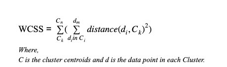
模型训练

先用 K=3 训练（Iris 已知有 3 个品种），排除 id 和 Species 列：

mldb=> SELECT kmeans('iris_model', 'iris_train_normalized', '*', 3
    USING PARAMETERS max_iterations=20, output_view='myKmeansView',
    key_columns='id', exclude_columns='Species, id');
kmeans
---------------------------
Finished in 11 iterations

肘部法确定最优 K

运行 K=1 到 K=8 计算 WSS（Within-Cluster Sum of Squares，簇内平方和）：

K (clusters)	Total WSS
1	313.5278
2	125.1907
3	78.0122
4	60.4885
5	59.4794
6	54.2670
7	39.8311
8	35.5652

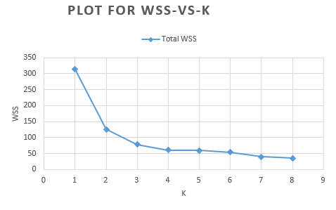
WSS 在 K=3 处出现明显拐点（肘部），K=3 到 K=4 下降幅度锐减，因此最优 K 值为 3。

模型摘要

mldb=> SELECT GET_MODEL_SUMMARY(USING PARAMETERS model_name='iris_model');

输出：

=======
centers
=======
sepal_length|sepal_width|petal_length|petal_width
------------+-----------+------------+-----------
  1.25019  |  0.15670  |   0.63945  |  0.56719
 -0.80817  |  0.89932  |  -1.31773  | -0.89097
  0.03038  | -0.75349  |   0.04167  |  0.08203

=======
metrics
=======
Evaluation metrics:
  Total Sum of Squares: 313.52783
  Within-Cluster Sum of Squares:
    Cluster 0: 26.084614
    Cluster 1: 24.722264
    Cluster 2: 27.205308
  Total Within-Cluster Sum of Squares: 78.012186
  Between-Cluster Sum of Squares: 235.51565
  Between-Cluster SS / Total SS: 75.12%

75.12% 的 Between-Cluster SS / Total SS 表明聚类效果良好。

应用到测试集

mldb=> SELECT id, Species,
    APPLY_KMEANS(Sepal_Length, Sepal_Width, Petal_Length, Petal_Width
        USING PARAMETERS model_name='iris_model', match_by_pos='true') AS predicted
    FROM iris_test_normalized;

部分输出（共 43 行）：

id  |  Species   | predicted
-----+------------+-----------
  4  | setosa     |         1
 15  | setosa     |         1
 20  | setosa     |         1
 54  | versicolor |         2
 56  | versicolor |         2
 59  | versicolor |         0
 99  | versicolor |         2
103  | virginica  |         0
127  | virginica  |         2
...  | ...        |       ...

模型评估

创建预测结果表

mldb=> CREATE TABLE iris_predicted_results AS
    SELECT *, CASE
        WHEN predicted=0 THEN 'virginica'
        WHEN predicted=1 THEN 'setosa'
        WHEN predicted=2 THEN 'versicolor'
        ELSE 'unknown'
    END AS predicted_species
    FROM (
        SELECT id, Species,
            APPLY_KMEANS(Sepal_Length, Sepal_Width, Petal_Length, Petal_Width
                USING PARAMETERS model_name='iris_model') AS predicted
            FROM iris_test_normalized
    ) foo;
CREATE TABLE

混淆矩阵

mldb=> SELECT CONFUSION_MATRIX(species, predicted_species
    USING PARAMETERS num_classes=3) OVER()
    FROM iris_predicted_results;

actual_class | class_index | predicted_0 | predicted_1 | predicted_2 | comment
--------------+-------------+-------------+-------------+-------------+------------------------------
virginica    |           0 |          11 |           4 |           0 |
versicolor   |           1 |           5 |          11 |           0 |
setosa       |           2 |           0 |           0 |          12 | Of 43 rows, 43 were used and 0 were ignored

模型正确预测了 34 个样本（virginica 11 + versicolor 11 + setosa 12），错误 9 个。

错误率

mldb=> SELECT ERROR_RATE(Species, predicted_species
    USING PARAMETERS num_classes=3) OVER()
    FROM iris_predicted_results;

class    |    error_rate     | comment
------------+-------------------+-----------------------------
setosa     |                 0 |
versicolor |            0.3125 |
virginica  | 0.266666666666667 |
           | 0.209302325581395 | Of 43 rows, 43 were used and 0 were ignored

平均错误率约 0.21（21%）。Setosa 完全正确，Versicolor 和 Virginica 各有一部分误判（因二者不可完全线性分离）。

总结

通过本文的完整实验，我们使用 Vertica 内置 ML 函数完成了：

1. Iris 数据集加载与训练/测试集拆分（TABLESAMPLE 30%）
2. 数据探索：异常值检测（DETECT_OUTLIERS）、归一化（NORMALIZE_FIT robust_zscore）、相关性分析（CORR_MATRIX）
3. 肘部法选择最优 K=3（WSS 表 K=1 至 K=8）
4. K-means 模型训练与摘要查看（get_model_summary，Between-Cluster SS / Total SS = 75.12%）
5. 测试集预测（APPLY_KMEANS）
6. 模型评估：混淆矩阵与错误率

扩展阅读

• Vertica K-Prototypes 聚类算法实战
• Vertica 内置 ML 速查表（v12.0.1）
• COPY 命令加载数据

参考链接

• Data Science Example - Iris dataset
• Iris Species Dataset - Kaggle
• Effect of Different Distance Measures on the Performance of K-Means Algorithm
• Evaluating and Validating Cluster Results
• Normalization based K means Clustering Algorithm
• Vertica Community Edition
• Vertica Documentation
• Vertica User Community